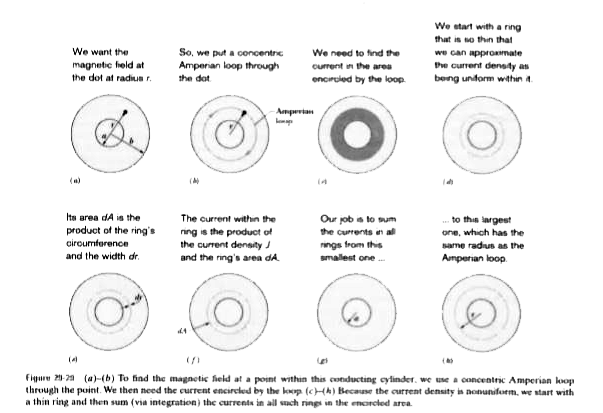
The point at which we want to evaluate `vecB` is inside the material of the conducting cylinder, between its inner and outer radii. We note that the current distribution has cylindrical symmetry (it is the same all around the cross section for any given radius). Thus, the symmetry allows us to use Ampere.s law of find `vecB` at the point. We first draw the Amperian loop shown in Fig. 29-29b. The loop is concentric with the cylinder and has radius `r=3.0cm` because we want to evaluate `vecB` at that distance from the cylinder.s central axis.
Next, we must compute the current `i_(enc)` that is encircled by the Amperian loop. However, we cannot set up a proportionality as in Eq. 29-38, because here the current is not uniformly distributed . Instead, we must integrate the current density magnitude from the cylinder.s inner radius a to the loop radius r, using the steps shown in Figs. 29-29c through h.
Calculations : We write the integral as
`i_(enc)=intJdA=int_(a)^(r )cr^(2)(2pirdr)`
`=2picint_(a)^(r )r^(3)dr=2pic[(r^(4))/(4)]_(a)^(r)`
`=(pic(r^(4)-a^(4))/(2))`.
Note that in these steps we took the differential area dA to be the area of the thin ring in Figs. 29-29d-f and then replaced it with its equivalent, the product of the ring .s circumference `2pir` and its thickness dr.
For the Amperian loop, the direction of integration indicated in Fig. 29-29b is (arbitarily) clockwise. Applying the right-hand rule for Ampere.s law to that loop, we find that we should take `i_(enc)` as negative because the current is directed out of the page but our thumb is directed into the page.
We next evaluate the left side of Ampere.s law as we did in Fig. 29-28, and we again obtain Eq. 29-37. Then Ampere.s law
`ointvecB*dcecs=mu_(0)i_(enc)`
gives us
`B(2pir)=-(mu_(0)pic)/(2)(r^(4)-a^(4))`
Solving for B and substituting known data yield
`B=-(mu_(0)c)/(4r)(r^(4)-a^(4))`
`=-((4pixx10^(-7)T*m//A)(3.0xx10^(6)A//m^(4)))/(4(0.030m))xx](0.030m)^(4)-(0.020m)^(4)]`
`=-2.0xx10^(-5)T`
Thus, the magnetic field `vecB` at a point `3.0cm` from the central axis has magnitude
`B=2.0xx10^(5)T`
and forms magnetic field lines that are directed opposite our direction of integration , hence counterclockwise in Fig. 29-29b