A thin rod of length L is lying along the x-axis with its ends at x=0 and x=L its linear (mass/length) varies with x as `k(x/L)^n`, where n can be zero of any positive number. If to position `x_(CM)` of the centre of mass of the rod is plotted against 'n', which of the following graphs best apporximates the dependence of `x_(CM)` on n?
A thin rod of length L is lying along the x-axis with its ends at x=0 and x=L its linear (mass/length) varies with x as `k(x/L)^n`, where n can be zero of any positive number. If to position `x_(CM)` of the centre of mass of the rod is plotted against 'n', which of the following graphs best apporximates the dependence of `x_(CM)` on n?
A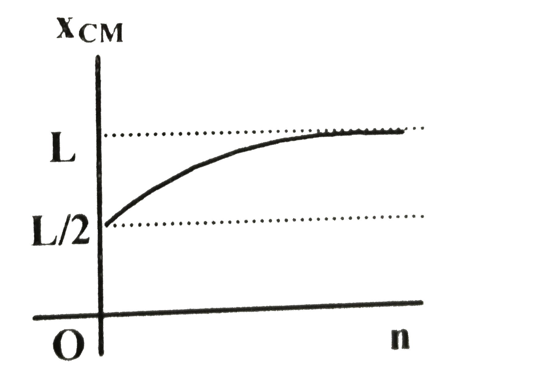
B
C
D
Text Solution
AI Generated Solution
The correct Answer is:
To solve the problem of finding the center of mass \( x_{CM} \) of a thin rod with a varying linear density, we will follow these steps:
### Step 1: Define the linear density
The linear density \( \lambda(x) \) of the rod is given by:
\[
\lambda(x) = k \left( \frac{x}{L} \right)^n
\]
where \( k \) is a constant, \( L \) is the length of the rod, and \( n \) can be 0 or any positive number.
### Step 2: Express the mass element
A small element of the rod \( dx \) at position \( x \) has mass \( dm \) given by:
\[
dm = \lambda(x) \, dx = k \left( \frac{x}{L} \right)^n dx
\]
### Step 3: Set up the center of mass formula
The center of mass \( x_{CM} \) is defined as:
\[
x_{CM} = \frac{\int_0^L x \, dm}{\int_0^L dm}
\]
### Step 4: Calculate the numerator
Substituting \( dm \) into the numerator:
\[
\int_0^L x \, dm = \int_0^L x \cdot k \left( \frac{x}{L} \right)^n dx = k \int_0^L x^{n+1} \frac{1}{L^n} dx
\]
This simplifies to:
\[
\frac{k}{L^n} \int_0^L x^{n+1} dx
\]
Calculating the integral:
\[
\int_0^L x^{n+1} dx = \left[ \frac{x^{n+2}}{n+2} \right]_0^L = \frac{L^{n+2}}{n+2}
\]
Thus, the numerator becomes:
\[
\int_0^L x \, dm = \frac{k L^{n+2}}{L^n (n+2)} = \frac{k L^2}{n+2}
\]
### Step 5: Calculate the denominator
Now, we calculate the denominator:
\[
\int_0^L dm = \int_0^L k \left( \frac{x}{L} \right)^n dx = k \int_0^L \frac{x^n}{L^n} dx = \frac{k}{L^n} \int_0^L x^n dx
\]
Calculating the integral:
\[
\int_0^L x^n dx = \left[ \frac{x^{n+1}}{n+1} \right]_0^L = \frac{L^{n+1}}{n+1}
\]
Thus, the denominator becomes:
\[
\int_0^L dm = \frac{k L^{n+1}}{L^n (n+1)} = \frac{k L}{n+1}
\]
### Step 6: Combine to find \( x_{CM} \)
Now substituting back into the formula for \( x_{CM} \):
\[
x_{CM} = \frac{\frac{k L^2}{n+2}}{\frac{k L}{n+1}} = \frac{L^2}{n+2} \cdot \frac{n+1}{L} = \frac{L(n+1)}{n+2}
\]
### Step 7: Analyze the relationship with \( n \)
From the expression \( x_{CM} = \frac{L(n+1)}{n+2} \), we can analyze how \( x_{CM} \) behaves as \( n \) changes:
- When \( n = 0 \):
\[
x_{CM} = \frac{L(0+1)}{0+2} = \frac{L}{2}
\]
- As \( n \to \infty \):
\[
x_{CM} \to L
\]
This indicates that as \( n \) increases, \( x_{CM} \) increases from \( \frac{L}{2} \) to \( L \).
### Conclusion
The graph of \( x_{CM} \) versus \( n \) will start at \( \frac{L}{2} \) when \( n = 0 \) and approach \( L \) as \( n \) increases. Thus, the graph will be an increasing function of \( n \).


Topper's Solved these Questions
Similar Questions
Explore conceptually related problems
A thin rod of length 6 m is lying along the x-axis with its ends at x=0 and x=6m. Its linear density *mass/length ) varies with x as kx^(4) . Find the position of centre of mass of rod in meters.
A rod of length L is placed along the x-axis between x=0 and x=L . The linear mass density (mass/length) rho of the rod varies with the distance x from the origin as rho=a+bx . Here, a and b are constants. Find the position of centre of mass of this rod.
A rod of length L is placed along the X-axis between x=0 and x=L . The linear density (mass/length) rho of the rod varies with the distance x from the origin as rho=a+bx. a.) Find the SI units of a and b b.) Find the mass of the rod in terms of a,b, and L.
A conductor of length L is placed along the x - axis , with one of its ends at x = 0 and the other at x = L. If the rate of flow of heat energy through the conduct is constant and its thermal resistance per unit length is also constant , then Which of the following graphs is/are correct ?
If linear density of a rod of length 3m varies as lambda = 2 + x, them the position of the centre of gravity of the rod is
A non–uniform thin rod of length L is placed along x-axis as such its one of ends at the origin. The linear mass density of rod is lambda=lambda_(0)x . The distance of centre of mass of rod from the origin is :
A rod of length L lies along the x-axis with its left end at the origin. It has a non-uniform charge density lamda=alphax , where a is a positive constant. (a) What are the units of alpha ? (b) Calculate the electric potential at point A where x = - d .
The density of a thin rod of length l varies with the distance x from one end as rho=rho_0(x^2)/(l^2) . Find the position of centre of mass of rod.
A uniform rod of length l is being rotated in a horizontal plane with a constant angular speed about an axis passing through one of its ends. If the tension generated in the rod due to rotation is T(x) at a distance x from the axis. Then which of the following graphs depicts it most closely?
A straight rod of length L has one of its end at the origin and the other at X=L . If the mass per unit length of the rod is given by Ax where A is constant, where is its centre of mass?